7 Excel tips & tricks from Alan Salmon

1.  Rounding Numbers

Excel provides a number of built-in worksheet functions for rounding numbers. The exact function you should use depends on exactly what you need to do with a value. The first worksheet function is ROUND. This function allows you to essentially round to any power of ten. The syntax is as follows:

       =ROUND(num, digits)

The num argument is the number you want to round, while digits indicate how many digits you want the result rounded to.

1. If digits is a positive value, then it represents the number of decimal places to use when rounding.
2. Thus, if digits is 3, then num is rounded to three decimal places.
3. If digits is zero, then ROUND returns a rounded whole number.
4. If digits is a negative number, then ROUND returns a number rounded to the number of tens represented by digits. Thus, if digits is –2, then ROUND returns a number rounded to the nearest 100.

Two other worksheet functions that return rounded values are ROUNDUP and ROUNDDOWN. These functions use the same arguments as ROUND and behave virtually identically. The only difference is that ROUNDUP always rounds num up, meaning away from 0. ROUNDDOWN is the opposite, always rounding down, toward 0.

2.  Paste Special – Multiply

If you have rather large pricing tables, you may not know the best way to update the prices by the ten per cent. Obviously, you could make a secondary table and then base the information in that table on a formula, such as =B3 * 1.1. This is actually more work than is necessary, however. There is a much quicker way to update values in a table by a uniform amount. Here are the steps:

1. Select an empty cell, somewhere outside the range used by your pricing table.
2. Enter the value 1.1 in the empty cell.
3. With the cell selected, press Ctrl+C to copy its contents to the Clipboard.
4. Select the entire pricing table. You should not select any headers or non-numeric information in the table.
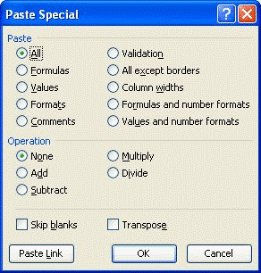
5. Choose the Paste Special option from the Edit menu.
6. Excel displays the Paste Special dialog box.
7. In the Operation area of the dialog box, select the Multiply option.
8. Click on OK.
9. Select the cell where you entered the value in step 2.
10. Press the Delete key.

You are done. All the values in your pricing table now show a ten percent increase from their previous values.

3.  Setting the Orientation of Cell Values             

Excel allows you to easily adjust how you want to display information in a cell. The Alignment icon in the Alignment group allows you to specify the orientation of the information within the cell (in which direction you want the text to be printed). You do this as follows: 

1. Select the cells whose orientation you want to change. 
2. In the Alignment group click on the  Click on the   icon. 
3. Select the Orientation you want to use from the list.
4. Click on OK. Your cell content is turned as you directed.
5. Format your columns so their width is better suited to the new text orientation.  

4.  Typing the Same Data in Multiple Cells

Have you ever had the need to type the same data in multiple cells in a worksheet? If so, you know that it can be time consuming if you have to manually enter the data in a lot of cells. Even copying and pasting can be time consuming. Here is a way to type the same data in multiple cells:

1. Select all of the cells that need to contain the same data. If the cells are consecutive you can click and drag to highlight them all, or you can hold down the CTRL button and click each individual cell. 
2. With all of the cells still highlighted, type the data you need repeated in all the cells in the last cell you selected.
3. After you type the data press CTRL and the Enter button. Your data should now be in all the cells you selected.

If you have multiple worksheets that need the same data in the same cells in each worksheet, you can automate this process even further by selecting each worksheet tab before you start selecting the cells in step #1 above. You can select multiple non-consecutive worksheet tabs by holding down CTRL and clicking on each tab, or if the tabs are consecutive you can click the first tab, hold down Shift, and then click the last tab. All tabs in between should also be highlighted. To deselect the tabs, click any other tab that is not in the group of tabs you are working on or right click a tab and select ungroup sheets.

5.  Backing Up Your Quick Access Toolbars 

The Quick Access Toolbar is a useful tool in Excel. If you get a new computer or your computer crashes you don't want to have to create your QATs from scratch. Here is how to backup your Quick Access Toolbar. 

1. Click the File tab on the ribbon. Click Options. Excel displays the Excel Options dialog box.
2. At the left side of the dialog box click Quick Access Toolbar. 
3. Click the Import/Export drop-down list at the bottom-right corner of the dialog box. Excel displays two options.
4. Choose Export All Customizations. Excel displays the File Save dialog box.
5. Using the controls in the dialog box, select a location where you want the backup file saved.
6. Click Save. Excel saves the customization file where you specified it in step 5.
7. Click on Cancel to dismiss the Excel Options dialog box.

The file created in step 6 is your backup file. You can store it where you store your other backups, and then reuse it by following the above steps, but choosing to import in step 4. 

6.  Summing Visible Cells

There are times when you need to add just the visible cells in an Excel worksheet. The Sum function in Excel adds all of the cells in a column or row, even if the columns and rows are hidden. The solution to just adding the visible cells is to use the =SUBTOTAL function. 

Assume that you have a column of numbers in column A from A1:A100 and that some of the cells are hidden. 

To get the total for just the visible cells you would use the following formula:  

                  =SUBTOTAL(109,A1:A100) 

The formula only calculates the sum of the visible cells in the range. And would you like to automatically sum a column or row from the keyboard? Here's how:    

Select the first empty cell at the bottom or to the right of the numbers you want to add.

• Select ALT+"="
• Press the Enter key
  The numbers will be summed.   

7.  Quickly Inserting the Date into a Worksheet

There are many times when you need to insert today's date into a worksheet. Here is how to do this: Select the cell where you want to enter today's date. Hold down the Ctrl key while you press the ; (Semi colon key) on your keyboard. Excel will enter today's date into the cell. 

Alan Salmon is recognized as Canada's leading analyst in accounting technology. As the founder of K2E Canada Inc., Alan has over 35 years of business, management systems, education and journalism experience.